

No correlation means two variables do not move together in a clear pattern. In a scatter plot, the points look randomly spread out instead of forming an upward or downward trend. Statistically, no correlation usually means the correlation coefficient is close to 0.
| Relationship type | Scatter plot pattern | Correlation coefficient (r) |
| Positive correlation | Points trend upward | r close to +1 |
| Negative correlation | Points trend downward | r close to -1 |
| No correlation | Points appear randomly scattered | r close to 0 |
Imagine you want to know if eating more apples makes you better at math. You collect data and place each result as a dot on a graph. In a no correlation scatter plot, the dots spread out randomly with no clear line or pattern. This tells you the two things are not related. When you spot no correlation, you avoid guessing connections that do not exist.
- You make better decisions by not assuming relationships.
- You focus only on data that matters for your business.
No-correlation scatter plots are just one type of relationship visualization. Explore additional scatter plot examples and learn how to create your own charts.
Understanding No Correlation Scatter Plot
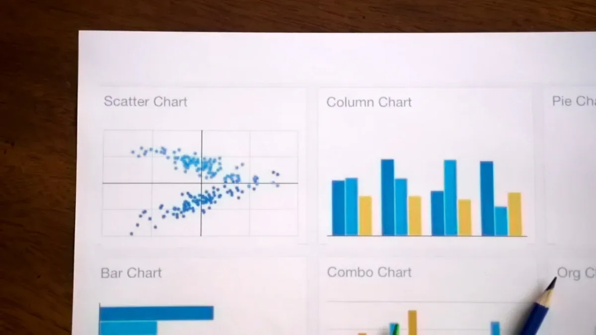
What Is a No Correlation Scatterplot?
You see a scatterplot when you want to compare two sets of numbers. In a no correlation scatter plot, the dots appear scattered all over the graph. The points do not form a line or curve. You cannot draw a trend line through them. This random spread means that changes in one variable do not affect the other. For example, if you plot shoe size against intelligence, the dots will not show any pattern. The lack of a pattern tells you there is no connection between the two things.
When you look at a scatterplot with no correlation, you notice that the data points do not cluster around any line. The graph does not show an upward or downward trend. The dots look like they are placed randomly. This visual clue helps you understand that the variables are unrelated.
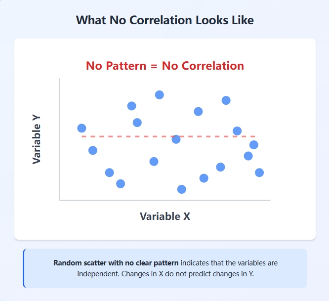
Tip: Always check for patterns in your scatterplot before making decisions. A random scatter means no correlation.
You can use statistical measures to confirm what you see. Pearson's correlation coefficient helps you check for a relationship. If the value is zero, it means there is no observable linear relationship. The table below shows how you can use these measures:
| Concept | Explanation |
|---|---|
| Zero Correlation (r=0) | Indicates no observable linear relationship between the two variables. |
| No Linear Trend Line | If no linear trend line can be drawn through the data, it confirms the absence of linear correlation. |
Why It Matters in Data Analysis
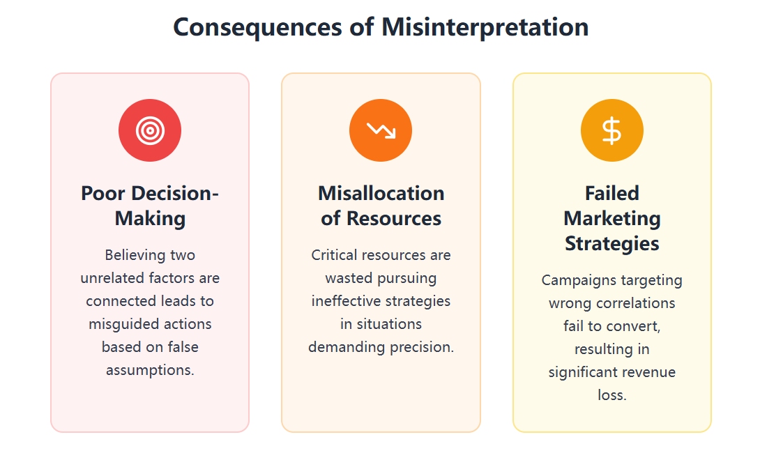
You need to recognize no correlation in your scatterplot to avoid mistakes. If you think two things are related when they are not, you might make poor choices. In business intelligence, this can lead to wasted time and money. Here are some problems that happen when you misinterpret a scatterplot with no correlation:
- Misguided actions leading to poor decision-making.
- Misallocation of resources, especially in critical situations.
- Failed marketing strategies resulting in loss of revenue.
You should always inspect your scatter plots carefully. Many people believe that a steep slope means strong correlation, but that is not true. The strength of a correlation depends on how closely the points cluster around a line, not the slope itself. Sometimes, scatterplots can mislead you if you do not consider outliers or nonlinear relationships. Visual inspection helps you spot these issues.
Data analysts use several methods to check for no correlation in large datasets. The table below lists some common approaches:
| Method | Description | Limitations |
|---|---|---|
| CUTIE | Detects false positives and negatives in correlation analysis. | Limited to identifying cases where significant correlations become non-significant. |
| Cook’s distance (Cook’s D) | Measures the effect of individual observations on the regression line. | Not symmetric with respect to 'x' and 'y' variables. |
| DFFITS | Identifies influential data points affecting regression results. | Similar limitations as Cook’s D; not symmetric. |
| Non-parametric methods | Spearman and Kendall rank-transform data to limit influential observation effects. | Less powerful than Pearson; should be used when data violates linear regression assumptions. |
| Log-transformations | Reduces skewness effects when using Pearson’s correlation. | Difficult to apply consistently across variables; selective transformation is challenging. |
You can use FineBI from FanRuan to make this process easier. FineBI lets you create scatterplots with a drag-and-drop interface. You can connect to many data sources and visualize your data in real time. The software helps you spot no correlation quickly. You can apply filters, check for outliers, and use built-in statistical tools. FineBI supports self-service analytics, so you do not need advanced technical skills. You can share your findings with your team and make better decisions.
Real-World No Correlation Scatterplot Examples
Website Visits vs Customer Satisfaction Score
Variables: Monthly unique website visitors (x-axis) vs. average CSAT score for that month (y-axis).
Expected pattern: Random scatter. High-traffic months do not consistently produce higher or lower satisfaction. Satisfaction is driven by product experience, support quality, and fulfillment — not visit volume.
Business takeaway: Investing in traffic acquisition alone will not improve CSAT. Diagnose satisfaction drivers separately from traffic metrics.
Employee ID Number vs Sales Performance
Variables: Sequential employee ID (x-axis) vs. quarterly revenue generated (y-axis).
Expected pattern: Pure random scatter. Employee IDs are arbitrary administrative identifiers with no logical connection to performance.
Business takeaway: Useful as a sanity check. If your scatter plot shows a pattern here, something is wrong with your data (e.g., IDs assigned chronologically correlating with tenure). Genuine no correlation confirms your axes are correctly specified.
Height vs. Exam Scores
Some people believe taller students perform better on exams. When you use a scatterplot to compare height and exam scores, you see no clear relationship. The points do not form a line or cluster. Research supports this observation:
- Height does not predict academic achievement.
- Any effect of height on test scores is extremely small.
- Over time, there is no pattern linking height changes to exam results.
Scatterplots help you and your students see that not all data pairs show a connection. FineBI’s data visualization tools make it easy to explore these relationships and teach the concept of no correlation scatter plot.
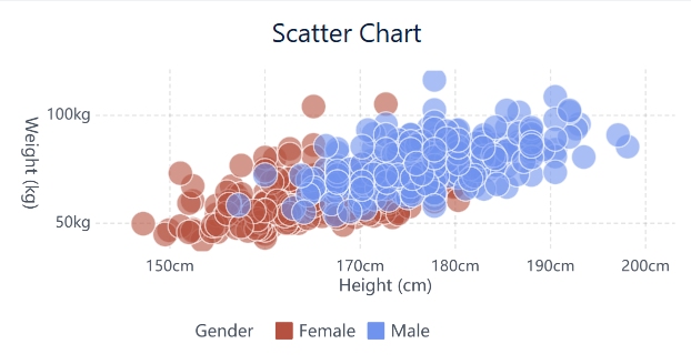
Office Floor Number vs Monthly Revenue
Variables: Floor number where a sales team sits (x-axis) vs. team monthly revenue (y-axis).
Expected pattern: No systematic trend. Teams on higher floors do not consistently outperform or underperform teams on lower floors.
Business takeaway: Physical location within a building is rarely a revenue driver. If analysis suggests otherwise, investigate confounders (e.g., senior teams occupying specific floors) before drawing conclusions.
Product SKU Number vs Return Rate
Variables: Numeric SKU identifier (x-axis) vs. return rate percentage (y-axis).
Expected pattern: Random scatter. SKU numbers are catalog identifiers, not product attributes. Return rates depend on category, price point, sizing accuracy, and quality — not numbering sequence.
Business takeaway: Analyze returns by product attributes (category, vendor, price tier), not by SKU number. This example reinforces the importance of choosing analytically meaningful variables.
Daily Meeting Count vs Deal Win Rate
Variables: Number of internal meetings held per day (x-axis) vs. deal win rate for deals active that week (y-axis).
Expected pattern: Weak or no correlation. More meetings do not reliably predict better outcomes; meeting quality, agenda focus, and participant relevance matter more than quantity.
Business takeaway: Meeting volume is a poor proxy for sales effectiveness. Track outcome-linked metrics (pipeline progression, stage conversion, stakeholder engagement) instead of activity counts.
Weight vs. Number of Pets Owned
You may think owning more pets could affect your weight or fitness. However, when you plot weight against the number of pets owned, the scatterplot shows no pattern. Studies with thousands of participants found no significant link between pet ownership and obesity or fitness. The lack of association holds true for all age groups and types of pets.
- Children with dogs are not fitter or less likely to be obese.
- Pet ownership does not change the odds of obesity.
FineBI allows you to visualize this data quickly. You can connect your survey results, drag the fields onto a scatterplot, and see the random distribution for yourself.

These examples demonstrate "no observable linear correlation in typical datasets." Specific organizations may find contextual relationships due to confounding variables. Always validate with your own data rather than assuming universal independence.
Download the Scatter Plot Example Dataset
Want to recreate these scatter plots yourself?
Download the sample dataset used in the examples and practice identifying positive, negative, and no-correlation relationships.
Dataset Includes:
- No correlation examples
- Positive correlation examples
- Negative correlation examples
- Multi-category scatter plot samples
- Ready-to-use CSV and Excel files
How to Tell If a Scatter Plot Has No Correlation
Use this checklist when evaluating any scatter plot:
- Visual inspection first: Do points form a discernible band, curve, or cluster? If they resemble a uniform cloud, suspect no correlation.
- Add a trendline: Insert a linear trendline with R² display. R² < 0.05 typically indicates negligible linear association.
- Calculate Pearson's r: Use built-in functions (=CORREL() in Excel, statistical packages in FineBI). Interpret magnitude alongside sample size.
- Check for outliers: A few extreme points can inflate or deflate r artificially. Remove or annotate outliers and recalculate.
- Test for nonlinearity: Fit a polynomial or LOESS curve. If a curved fit explains significantly more variance than a linear fit, the relationship may be nonlinear despite r ≈ 0.
- Segment the data: Split by category, time period, or cohort. Apparent no correlation in aggregate may mask strong correlations within subgroups (Simpson's paradox).
- Validate with domain knowledge: Does a plausible mechanism connect these variables? Statistical results should be interpreted alongside subject-matter expertise.
Skipping visual inspection and relying solely on r is the most common analytical error. Always plot before you compute.
How to Create a Scatter Plot Using the Example Dataset
After understanding how no-correlation scatter plots work, the next step is to create your own chart and explore the data visually.
You can use either Excel or FineBI to build the chart in just a few minutes.
Create a Scatter Plot in Excel
Excel is one of the easiest tools for creating scatter plots and identifying whether two variables are correlated.
Step 1: Download the Example Dataset
Download the sample scatter plot dataset and open it in Excel.
Download Scatter Plot Dataset →
Step 2: Select the Data
Highlight the two numerical columns you want to compare. For example:
- Advertising Spend
- Monthly Revenue
or
- Study Hours
- Exam Scores
Step 3: Insert a Scatter Plot
Navigate to:
Insert → Charts → Scatter → Scatter with Only Markers
Excel will automatically generate a scatter plot using the selected data.
Step 4: Interpret the Pattern
Observe how the data points are distributed:
- Upward trend → Positive Correlation
- Downward trend → Negative Correlation
- Random distribution → No Correlation
Step 5: Customize the Chart
To improve readability:
- Add chart titles
- Label the X and Y axes
- Adjust marker size and color
- Add a trendline if needed
By experimenting with different variables in the sample dataset, you can quickly learn how different correlation patterns appear in practice.
How to Visualize Correlation in FineBI
Excel works for small sample datasets. But when your data comes from CRM, sales systems, marketing platforms, or operational databases, FineBI helps you build scatter plots from live business data, filter by segment, compare multiple variables, and quickly check whether a relationship is positive, negative, or close to no correlation.
| Task | Excel | FineBI |
| Small sample scatter plot | Good fit | Also supported |
| Live business data | Manual import | Connects to business data sources |
| Segment comparison | Manual filtering | Interactive filters and drill-downInteractive filters and drill-down |
| Team sharing | File-based | Shared dashboard |
| Ongoing monitoring | Manual refresh | Scheduled or live dashboard updates |
Step 1: Download the Example Dataset
Start by downloading the scatter plot sample dataset.
Download Scatter Plot Dataset →
Step 2: Import the Dataset into FineBI
Upload the Excel or CSV file into FineBI and create a new analysis project.
Step 3: Create a Scatter Plot
From the visualization panel:
- Drag one numerical field to the X-axis.
- Drag another numerical field to the Y-axis.
- Select Scatter Plot as the chart type.
FineBI automatically generates the visualization.
Step 4: Add Dimensions and Filters
To gain deeper insights, you can:
- Color points by category
- Filter by date, region, or product
- Compare multiple groups within a single chart
This helps reveal hidden relationships that may not be obvious in a basic scatter plot.
Step 5: Turn Analysis into a Dashboard
Once your scatter plot is complete, you can combine it with:
- KPI cards
- Trend charts
- Bar charts
- Geographic maps
to create a complete analytical dashboard.
Why Use FineBI for Scatter Plot Analysis?
Compared with spreadsheet-based analysis, FineBI offers:
- Interactive filtering and drill-down
- Faster exploration of large datasets
- Automated dashboard creation
- Multi-source data integration
- Easy sharing across teams
Whether you're learning data visualization or building business reports, FineBI helps you move from static charts to interactive analysis.
After analysts identify weak or no correlation in FineBI, Dora can help summarize the finding, generate follow-up questions, and suggest which variables to test next — turning exploratory analysis into structured investigation workflows.

Continue Reading About Data Visualization
How to Create Good Data Visualization Examples for Beginners
Histogram vs Bar Graph: How They Enhance Data Visualization
Understanding Component Bar Chart in Data Visualization
Frequently asked questions
You see dots scattered randomly across the graph. The points do not form any line or curve. No pattern appears, so you cannot predict one variable from the other.